parallel dplyr

May 24, 2017 · 2 min read · R ·

Introduction

I’m a big fan of the R packages in the tidyverse and dplyr in particular for performing routine data analysis. I'm currently working on a project that requires fitting dose-repsonse curves to data. All works well when the amount of data is small but as the dataset grows so does the computational time. Fortunately there’s a library (multidplyr) to perform dplyr operations under parallel conditions. By way of example we’ll create a set of dummy data and compare curve fitting using dplyr and multidplyr.

The dataset used is the spinach dataset that comes with the drc package. It's a data frame containing 105 observations in 5 groups. Each group consists of 7 concentrations run in triplicate. To compare dplyr and multidplyr we'll take these measurements and copy them 1000 times with some jitter.

Code

 1
 2## Libraries
 3library(drc)
 4library(dplyr)
 5library(multidplyr)
 6library(microbenchmark)
 7library(ggplot2)
 8library(tidyr)
 9
10## Create a dummy dataset
11data <- spinach
12for (i in 1:1000) {
13  addData <- spinach
14  addData$CURVE <- addData$CURVE + 5 * i
15  addData$SLOPE <- sapply(addData$SLOPE, function(x) jitter(x, factor = 10))
16  data <- rbind(data, addData)
17}
18
19## Define some functions
20makeFit <- function(d) {
21  tryCatch(drm(SLOPE ~ DOSE, data = d, fct = LL.4()), error = function(e) NA)
22}
23
24fit_dplyr <- function(data, n) {
25  data %>%
26    filter(CURVE <= n) %>%
27    group_by(CURVE) %>%
28    do(fit = makeFit(.))
29}
30
31fit_multidplyr <- function(data, n) {
32  data %>%
33    filter(CURVE <= n) %>%
34    partition(CURVE) %>%
35    cluster_copy(makeFit) %>%
36    cluster_library('drc') %>%
37    do(fit = makeFit(.)) %>%
38    collect(unique_indexes = 'CURVE')
39}
40
41## Benchmark our data
42microbenchmark(fit_dplyr(data, 10), times = 3)
43microbenchmark(fit_dplyr(data, 100), times = 3)
44microbenchmark(fit_dplyr(data, 1000), times = 3)
45microbenchmark(fit_dplyr(data, 5000), times = 3)
46microbenchmark(fit_multidplyr(data, 10), times = 3)
47microbenchmark(fit_multidplyr(data, 100), times = 3)
48microbenchmark(fit_multidplyr(data, 1000), times = 3)
49microbenchmark(fit_multidplyr(data, 5000), times = 3)
50
51## Conclude with a table and graph
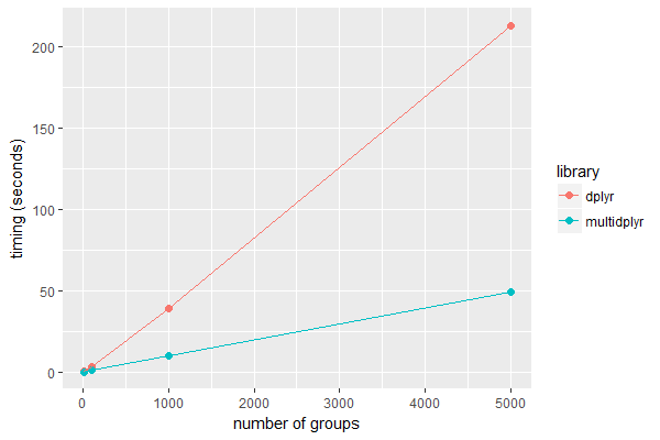
52df.graph <- data.frame(n = rep(c(10, 100, 1000, 5000), 2), library=rep(c('dplyr', 'multidplyr'), each=4), timing=c(0.20, 3.04, 39.07, 212.89, 0.13, 1.13, 10.13, 49.29))
53
54ggplot(df.graph, aes(x=n, y=timing, colour=library)) +
55  geom_point(size = 2) +
56  geom_line() +
57  labs(x = 'number of groups', y = 'timing (seconds)')
58
59df.table <- df.graph %>%
60  spread(library, timing) %>%
61  mutate(enhancement = round(dplyr / multidplyr, 2))
62

Conclusion

In this case, multidplyr runs up to 4.3 times faster on a 16 core PC. The speed enchancement increases with increasing size of the dataset.

n	dplyr (secs)	multidplyr (secs)
10	0.20	0.13
100	3.04	1.13
1000	39.07	10.13
5000	212.89	49.29