Beer Trip Around the World
The traveling salesperson problem (TSP) is an NP-complete problem that asks given a list of cities, what's the shortest path that can be taken so that each city is visited once and you end up back where you started. Exact solutions to the problem exist but they become impractical as soon as the number of cities increases above 20 therefore approximations are generally performed that yield a suitable, if not best, solution.
Here we take a fun approach from a thought experiment. What if I could idenfity the best beers in the World and drink them in the breweries in which they are brewed. With a limited time and budget, wouldn't this be a traveling salesperson problem? With this is mind I quickly drew up the following solution using the {TSP} R package.
Step 1 - Gather and wrangle the data
Data were retrieved from Kaggle. Kaggle contains a few beer datasets but the one chosen (https://www.kaggle.com/ehallmar/beers-breweries-and-beer-reviews) contains beers, reviews and breweries, making our life much easier. Once data were downloaded we could identify top-rated beers and join brewery details to produce a single, neat data frame.
 1library(readr)
 2library(dplyr)
 3library(here)
 4
 5## read in beer data
 6df_beers <- read_csv(here("data/beers.csv"))
 7
 8## read in beer ratings
 9df_ratings <- read_csv(here("data/reviews.csv"))
10
11## read in breweries
12df_breweries <- read_csv(here("data/breweries.csv"))
13
14## summarize ratings by beer and sort
15df_rating_summary <- df_ratings %>%
16  group_by(beer_id) %>%
17  summarise(rating = mean(score, na.rm = TRUE)) %>%
18  arrange(desc(rating)) %>%
19  filter(rating >= 4.75)
20
21## add ratings summary to beer data frame
22df_beer_ratings <- df_beers %>%
23  right_join(df_rating_summary, by = c("id" = "beer_id")) %>%
24  filter(retired == FALSE)
25
26## add brewery details
27df_beer_ratings <- df_beer_ratings %>%
28  select(id, beer=name, brewery_id, rating, abv) %>%
29  left_join(df_breweries %>% select(id, brewery=name, city, state, country), by = c("brewery_id" = "id")) %>%
30  arrange(desc(rating))
31
32## limit to single occurrence of each brewery
33df_beer_ratings <- df_beer_ratings %>%
34  group_by(brewery_id) %>%
35  arrange(desc(rating), desc(abv)) %>%
36  slice(1) %>%
37  ungroup()
Step 2 - Convert locations to longitude/latitude
Now we have a table with locations we can easily convert the locations to longitude/latitude values which will be used to calculate distances. First we need to convert the county code from a two-character abbreviation and then we can use {tidygeocoder} to convert to longitude and latitude.
 1library(countrycode)
 2library(tidygeocoder)
 3
 4## build city addresses
 5df_beer_ratings <- df_beer_ratings %>%
 6  mutate(country_name = countrycode(country, origin = "iso2c", destination = "country.name")) %>%
 7  mutate(address = if_else(country == "US", paste(city, state, "USA", sep = ", "), paste(city, country_name, sep = ", ")))
 8
 9## take the first 300 locations
10df_use_locations <- df_beer_ratings %>%
11  slice(1:300)
12
13## determine longitude and latitude
14df_address <- geo(df_use_locations$address, method = "cascade")
15
16## bind locations to data frame
17df_use_locations <- bind_cols(df_use_locations, df_address %>% select(lat, long)) %>%
18  filter(!is.na(lat), !is.na(long))
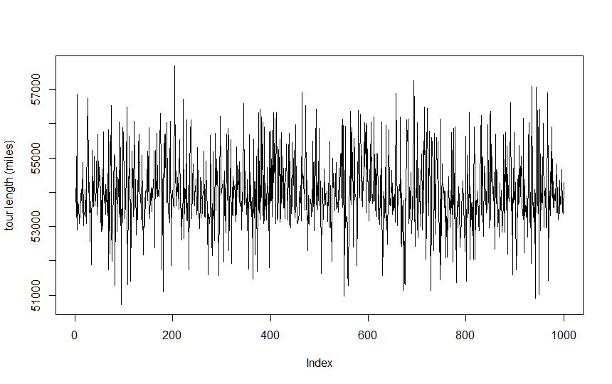
Step 3 - Build a distance matrix and run TSP
Once we have a list of longitude/latitude pairs we can build a distance matrix of the distances between each location (default measurement = meters). From this we can solve the traveling salesperson problem. In this example TSP is solved 1000 times and the distance (in miles) plotted. Finally, the shortest tour is plotted using leaflet.
 1library(geodist)
 2library(TSP)
 3library(leaflet)
 4
 5## build a distance matrix
 6dist_m <- geodist(df_use_locations %>% select(lat, long), measure = "geodesic")
 7
 8## build TSP and solve 1000 times
 9set.seed(1234)
10tsp <- TSP(dist_m, labels = df_use_locations$address)
11beer_trip <- lapply(seq(1000), function(x) solve_TSP(tsp))
12
13## plot results and identify the shortest tour
14tours <- sapply(beer_trip, tour_length) / 1609.34
15plot(tours, type = "l", ylab = "tour length (miles)")
16shortest_tour <- which.min(tours)
17
18
19## reorder locations according to shortest tour
20ref_order <- unlist(lapply(beer_trip[[shortest_tour]], function(x) x), use.names = FALSE)
21df_solution <- df_use_locations[ref_order, ]
22df_solution[nrow(df_solution) + 1, ] <- df_solution[1, ]
23
24## plot tour on leaflet map
25leaflet(data = df_solution) %>%
26  addTiles() %>%
27  addCircleMarkers(~long, ~lat, popup = ~brewery, radius = 2, color = "red") %>%
28  addPolylines(~long, ~lat, weight = 4)
Conclusion
The data may or may not be the best quality but the concept holds true. Total length of trip (between 297 locations) = 50718 miles.